SITCOMTN-104: WET-001 - Optical State Measurement Verification Test

• Guillem Megias Homar

Latest Revision: 2024-01-26

Note

This technote is a work-in-progress.

1 Abstract

This technote covers WET-001 Test from the AOS Commissioning Test List. It aims to validate that the AOS is able to retrieve the optical state injected into the system. This technote will eventually cover multiple different conditions (different filters, different rotation angles). For now, it only covers the case of the r-band filter and the 0 degree camera rotation angle.

The notebook used to generate the data for this technote can be found in this technote repository.

2 Background

For that process to be successful the AOS relies in two different components:

1. Wavefront Estimation Pipeline algorithm:

   The errors in estimating the wavefront zernikes influence the accuracy of the retrieved optical state. This process is also studied in other tehcnotes. The three approaches that can be considered when estimating the wavefront are:

   1. Danish

   2. TIE

   3. ML

2. Optical state estimation:

   Once the wavefront is estimated, the optical state is retrieved through the sensitivity matrix. The process involves the pseudo-inverse of the sensitivity matrix (\(A\)) and the truncation on those degenerate degrees of freedom.

   For reference, we include the main equation involved in this process. Here, \(y\) is the estimated zernikes minus the intrinisic zernikes in microns, and \(x\) is the retrieved optical state in the basis of degrees of freedom (microns or arcsec, depending on the degre e of freedom). Finally, rcond refers to the threshold used to truncate the singular values of the degrees of freedom.

   x = pinv(A, rcond=1e-4) @ y
   

3 Simulation

For a set of 100 different optical states (degree of freedom states) we generate the corner sensor images. The optical states are generated following the process described in [1]. Below two images are shown, one for the injected degree of freedom state, and one for the simulated corner image:

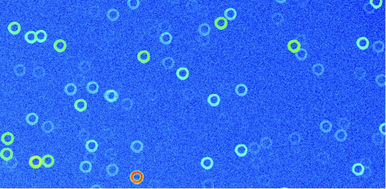
Figure 1 Figure 1: Simulated image in corner R00 sensor for the first optical state.

Figure 2 Figure 2: First optical state of the 100 simulated states.

The images were simulated with the following conditions:

RA	Dec	Seeing
15:17:00.75	-9:22:57.7	0.3 arcsec

The images can currently be found in the personal butler of the author (/sdf/data/rubin/user/gmegias/projects/commissioning_sims/butler_wet001). Once the technote has been peer-reviewed and the data is vetted, it will be transferred to the AOS commissioning shared butler.

4 Results

4.1 Wavefront estimation

So far we focus on running the WEP pipeline using the baseline TIE algorithm. The results shown below include the cutout donuts and estimated zernikes versus true zernikes for the first optical state.

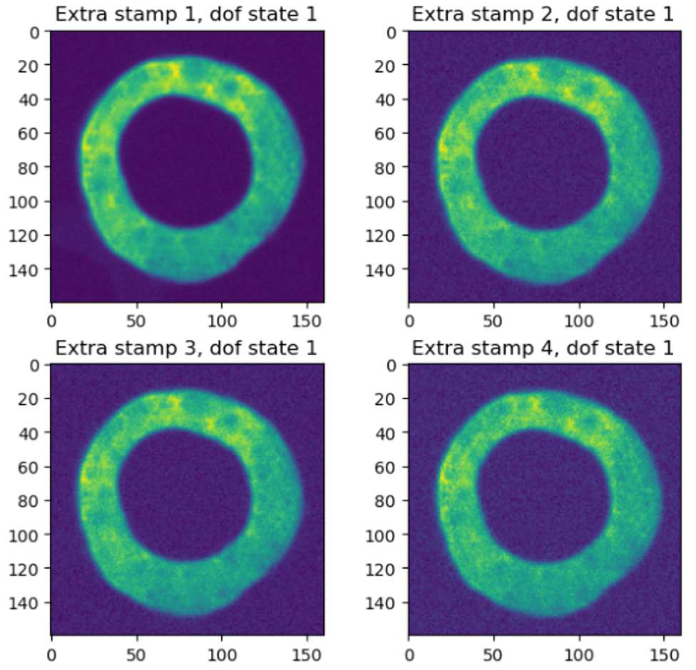
Figure 3 Figure 3: Cutout donuts for the first optical state.

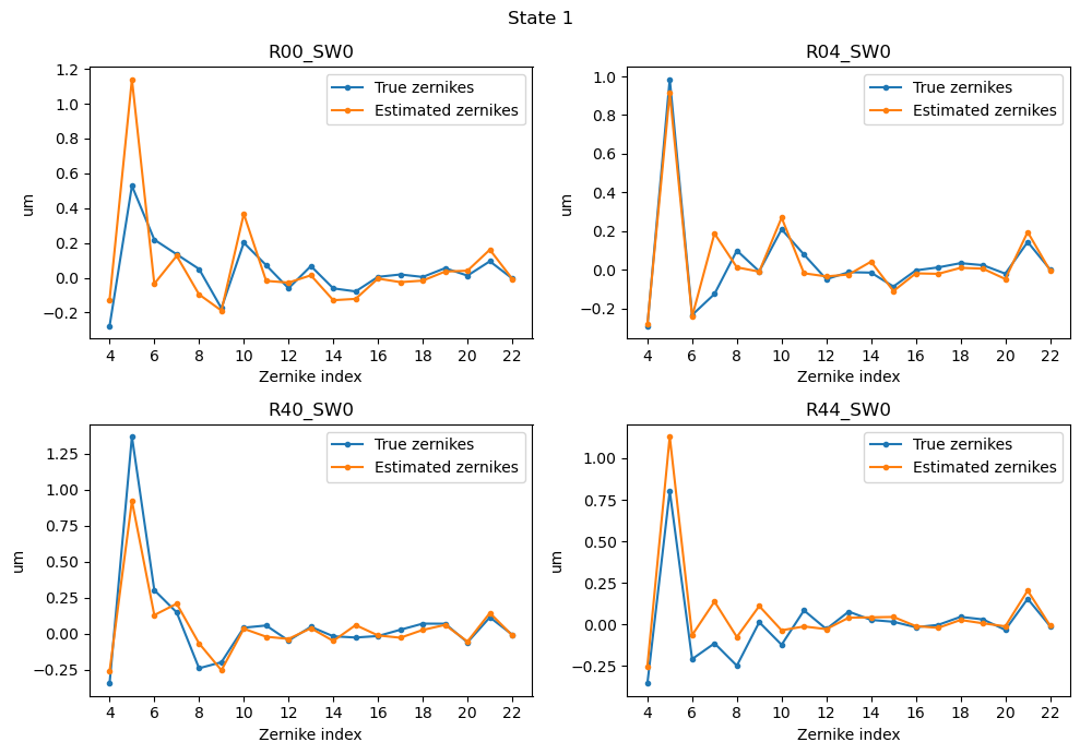
Figure 4 Figure 4: Estimated zernikes versus true zernikes for the first optical state.

Finally, we also include the median error and std of the estimated zernikes error for the 100 different optical states. The results are shown in the plot below:

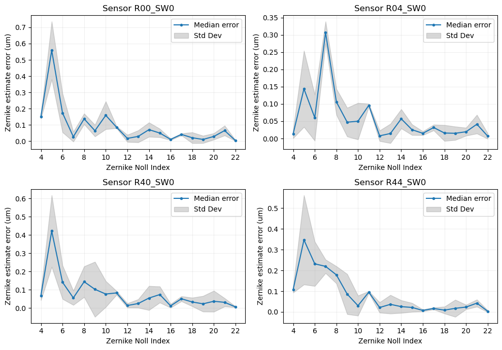
Figure 5 Figure 5: Estimated zernikes error statistics

4.2 Optical state estimation

Finally, keeping in mind that as shown above our estimates of the wavefront are not perfect, we proceed to retrieve the optical state for the 100 different optical states. The results for the first simulated optical state are shown below. We include a comparison between the injected optical state versus the retrieved one, as well as comparison of the reconstructed zernikes (obtained multipliying the sensitivity matrix by the estimated optical state) versus the true zernikes and the WEP estimated ones.

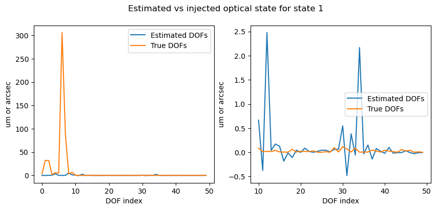
Figure 6 Figure 6: Injected optical state versus retrieved optical state for the first simulated optical state.

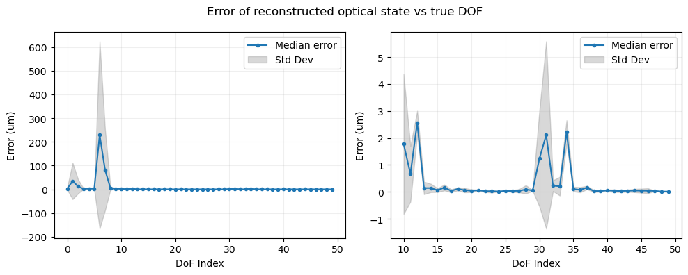
Figure 7 Figure 7: Reconstructed zernikes versus true zernikes and estimated zernikes for the first simulated optical state.

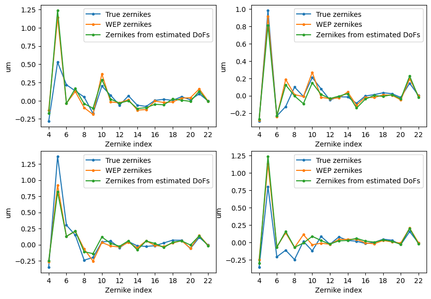
Figure 8 Figure 7: Reconstructed zernikes versus true zernikes and estimated zernikes for the first simulated optical state.

Finally, we also include the median error and std of the reconstructed zernikes versus the estimated WEP zernikes. The results are shown in the plot below:

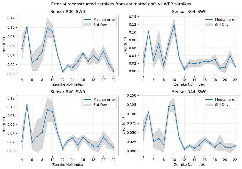
Figure 9 Figure 8: Reconstructed zernike vs WEP zernike error statistics.

References

[1]

John Franklin Crenshaw, Andrew Connolly, Joshua Meyers, Bryce Kalmbach, Guillem Megias Homar, Tiago Ribeiro, Krzysztof Suberlak, Sandrine Thomas, and Te-Wei Tsai. Ai Wavefront Estimation for the Rubin Observatory Active Optics System. Bulletin of the AAS, jan 31 2023. https://baas.aas.org/pub/2023n2i207p07.